46. Title : From common properties to Synthetic Lethality prediction

46.1. Date

29042020

46.2. Goal

• To explore the data available on interactors partners and go terms of the budding yeast genes, to see the correlations between the common go terms and common interaction partners between two genes and the type of pairwise interaction .

• Here I am focused on synthetic lethality interactions and negative interactions as the positive classes. The rest of the interactions are seen as the opposite class.

46.3. Method

• Marginal features,i.e, summary of the variable

  • common interaction partners between two genes

  • common Go terms between two genes

• Correlations explored using Python

• Test the capability of applying some methods to fit the data and make some predictions

46.4. Results

THE CODE THAT GENERATES THESE PLOTS IS IN THIS GITHUB REPO

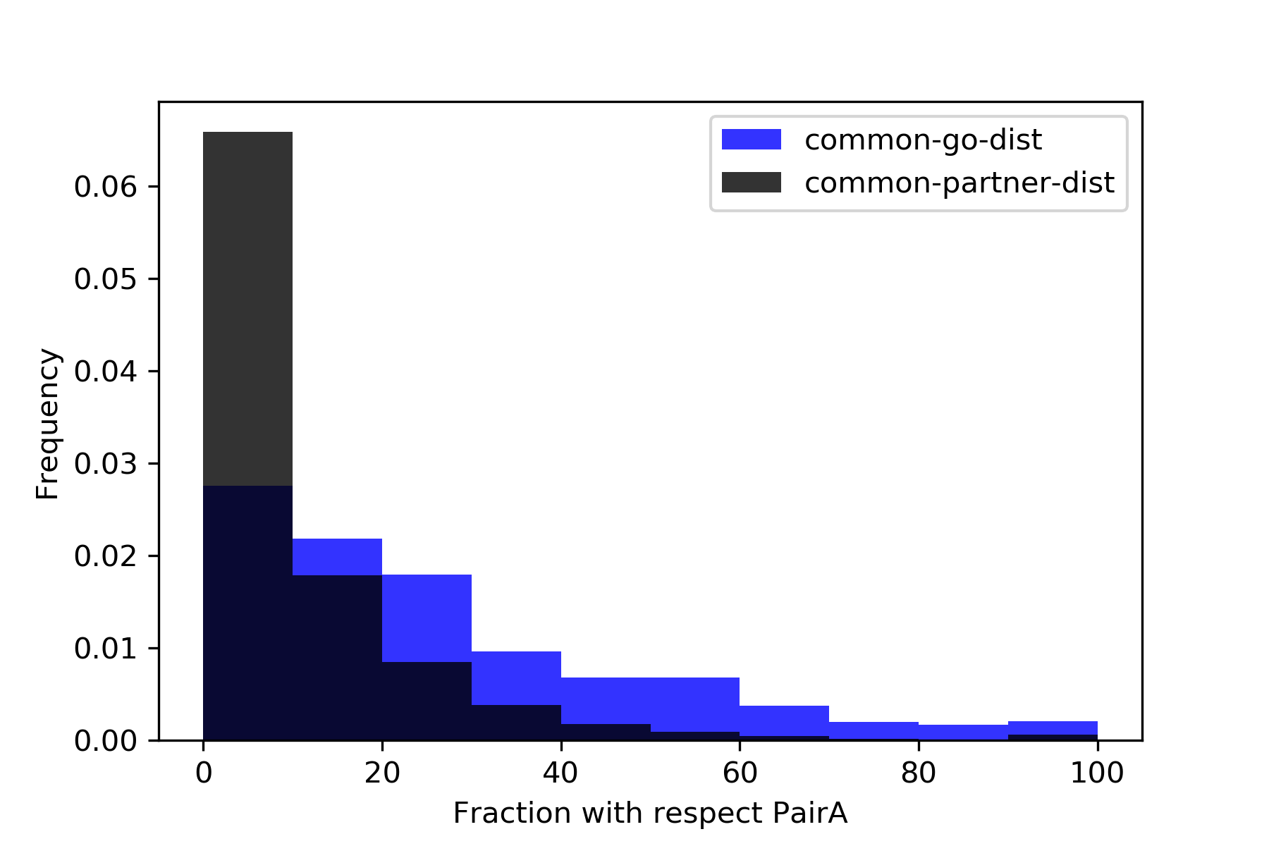
{#fig:hist}

46.4.1. Only taking Synthetic lethals interaction as the target one over 1000 genes

1. Variables explained:

   • n_common= # of common interactors between pairA(query) and pairB(target)

   • fraction of common partners :

   \(\frac{n_{common}}{len(partners of pair A)}\)

   • fraction of common go= # of common go terms between pairA(query) and pairB(target)

   • type-code : 0 if type of interaction is not SL,1 if type of interaction is SL

	fraction-of-common-partners	fraction-of-common-go
corr with type-code	0.07576721633851422	0.04771031641861598
p-value	2.3182505415835613e-75	6.807479091460884e-31

1. Interpretation

   • There is a poor correlation between the fact of being synthetic lethals and the common properties. However all the poor correlations are highly significant and positive.

46.4.2. Taking Negative Genetic and Synthetic lethals interaction as the target one over 1000 genes

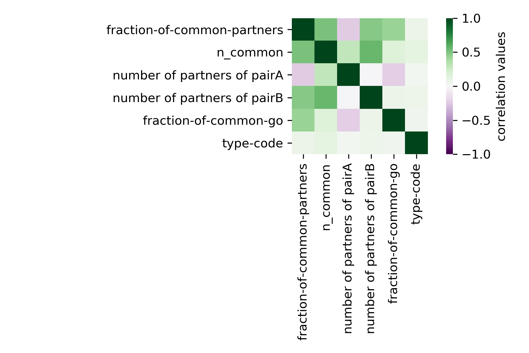
{#fig:correlation-NG}

{#fig:violinplots-NG}

• Interpretation

  • After considering also gene pairs annotated to interact negatively in the same class as SL, the correlation gets a bit better.

  • We can see that the fraction of common go terms correlates negatively with the type of interaction. This reads as: As the code increase(to 1,in this case SL or negative) the fraction of common go terms decrease in the pair and viceversa.

  • We can see in the table below that actually the negative correlation with common go terms and the type of interaction is highly significant. This could be a confirmation that as more overlapping biophysical properties two genes have , the less the chances those genes interact negatively or in the worse case being synthetic lethals.

	fraction-of-common-partners	fraction-of-common-go
corr with type-code2	0.005049651435548733	-0.06558633110815931
p-value[^1]	0.2215193380382011	6.844074442839657e-57
[^1]: The p-value roughly indicates the probability of an uncorrelated system producing datasets that have a Pearson correlation at least as extreme as the one computed from these datasets. The p-values are not entirely reliable but are probably reasonable for datasets larger than 500 or so.

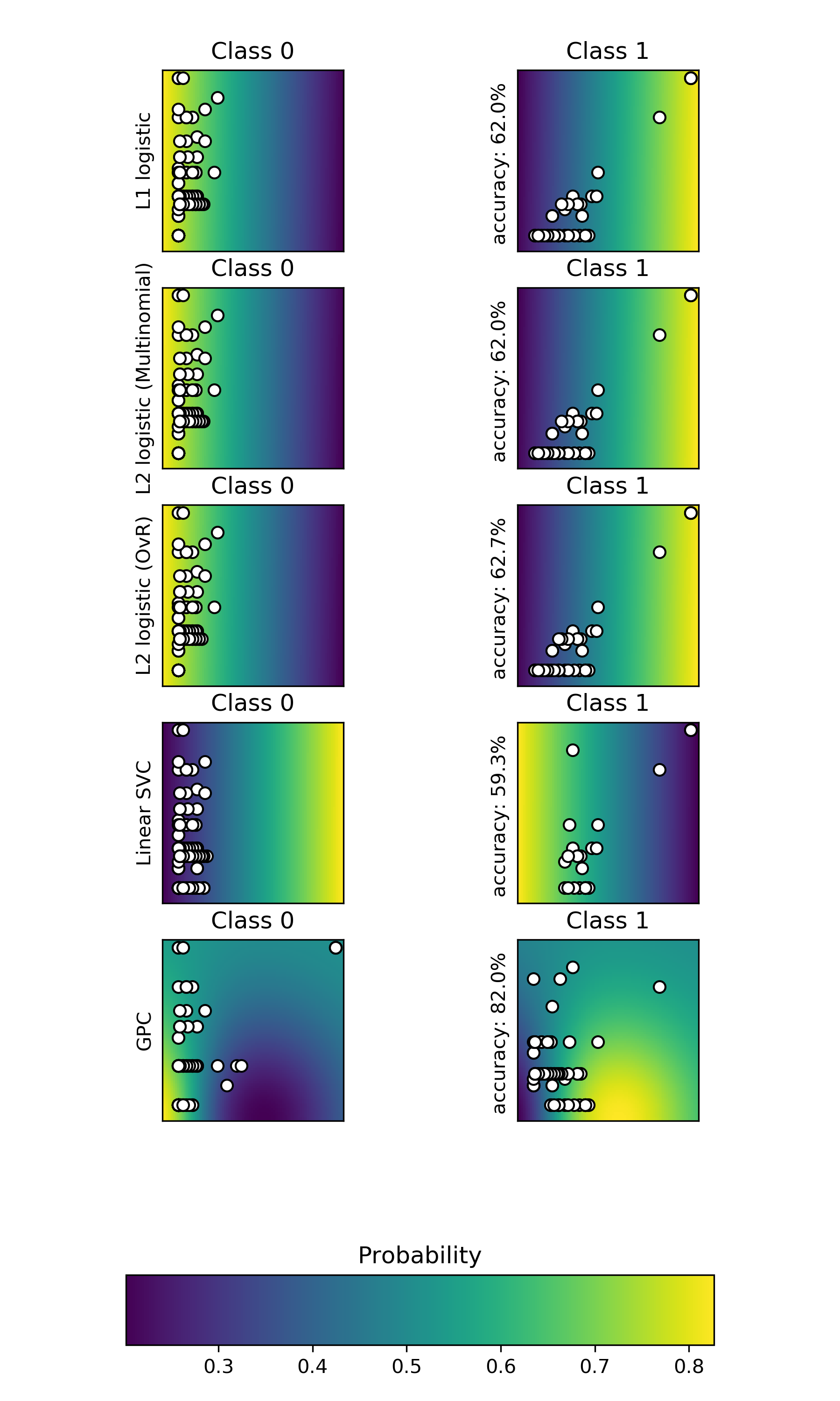
46.4.3. Comparison on learning algorithms to predict the probability that the type of interaction is 0 or 1, that is , nonSL or SL.

46.5. Conclusions

1. Common go terms and common interaction partners ovwer 1000 shows still a general poor correlation with SL and non SL pairs.

2. Perhaps I need to increase the sample size to more genes.

3. When I do a less astringent SL class by including also negative interactors, what happens is that the correlation with being SL and having common go terms is negative but low (~6%) , and this is highly significant (~10\(^{-57}\)). This means that the chances of having 0% correlation with this dataset is exteremely low, almost imposible.

---

2

The Pearson correlation coefficient measures the linear relationship between two datasets. Strictly speaking, Pearson’s correlation requires that each dataset be normally distributed. Like other correlation coefficients, this one varies between -1 and +1 with 0 implying no correlation. Correlations of -1 or +1 imply an exact linear relationship. Positive correlations imply that as x increases, so does y. Negative correlations imply that as x increases, y decreases.